Hpcviewer#
Overview#
HPCToolkit provides the hpcviewer (Adhianto, Mellor-Crummey, and Tallent 2010; Tallent et al. 2011) graphical user interface for interactive examination of performance databases.
hpcviewer presents a heterogeneous
calling context tree that spans both CPU and GPU contexts, annotated
with measured or derived metrics to help users assess code performance
and identify bottlenecks.
The database generated by hpcprof consists of 4 dimensions:
Execution context (also called execution profile), which includes any logical threads (such as OpenMP, pthread, and C++ threads), MPI processes, and GPU streams.
Time, which represents the timeline of the program’s execution. This time dimension is only available if the application is profiled with traces enabled (
hpcrun-toption).Call-path, which depicts a top-down path in a calling-context tree.
Metric, which constitutes program measurements performed by
hpcrunsuch as cycles, number of instructions, stall percentages, and derived metrics such as ratio of idleness.
To simplify performance data visualization, hpcviewer restricts
the display of two dimensions at a time: the Profile View displays
pairs of (call-path, metric) or (execution context,
metric) dimensions and the Trace View visualizes the
behavior of execution contexts over time.
The table below summarizes views supported by hpcviewer.
View |
Dimension |
Note |
|---|---|---|
Profile - Metric view |
Call-path x Metrics |
display the tree and its associated metrics |
Profile - Thread view |
Call-path x Metrics |
display the tree and its metrics for a set of execution contexts |
Profile - Graph view |
Execution contexts x Metric |
display a metric of a specific tree node for all execution contexts |
Trace - Main view |
Execution contexts x Time |
display execution context behavior over time |
Trace - Depth view |
Call-path x Time |
display call stacks over time of an execution context |
Note that in the Profile view, GPU stream execution contexts are not shown in this view; metrics for a GPU operation are associated with the calling context in the thread that initiated the GPU operation (Section Thread View). In the Trace view, GPU streams have their trace lines independently from their host, allowing for the traces between hosts and devices to be separated.
Downloading#
While you can build your own copy of HPCToolkit’s hpcviewer graphical user interface,
we recommend downloading a binary release at https://hpctoolkit.org/download.html.
Pre-built packages are available for Linux (x86_64, aarch64, ppcle), MacOS (aarch64, x86_64), and Windows (x86_64).
Note
Trace views previously provided by HPCToolkit’s hpctraceviewer interface have been integrated into hpcviewer since its 2020.12 release.
Building from Source#
Source code for HPCToolkit’s hpcviewer graphical user interface is available at hpctoolkit/hpcviewer.git. Clone a copy with git.
Building hpcviewer requires maven.
You can download a copy of maven with Spack.
To build hpcviewer on your platform of choice, follow the directions in its README.md on Gitlab.
Launching#
Requirements to launch hpcviewer:
On all platforms: Java 17 or newer (up to Java 21).
On Linux: GTK 3.20 or newer.
hpcviewer can be launched from a command line (Linux platforms) or by clicking the hpcviewer icon (for Windows, Mac OS X, and Linux platforms).
The command line syntax is as follows:
hpcviewer [options] [<hpctoolkit-database>]
Here, <hpctoolkit-database> is an optional argument to load a database automatically.
Without this argument, hpcviewer will prompt for the location of a database. Possible options for hpcviewer are shown below:
-h, --helpPrint a help message.
-jh, --java-heapsizeSet the JVM maximum heap size for this execution of
hpcviewer. The value of size must be in megabytes (M) or gigabytes (G). For example, one can specify a size of 3 gigabytes as either 3076M or 3G.-v, --versionPrint the current version
On Linux, when hpcviewer is installed using its install.sh script, one can specify the maximum size for the Java heap on the current platform. When analyzing measurements for large and complex applications, it may be necessary to use the --java-heap option to specify a larger heap size for hpcviewer to accommodate many metrics for many contexts.
On macOs and Windows, the value of JVM maximum heap size is stored in hpcviewer.ini file, specified with -Xmx option.
On macOS, this file is located at hpcviewer.app/Contents/Eclipse/hpcviewer.ini.
Limitations#
Some important hpcviewer limitations are listed below:
Limited number of metric columns.
With a large number of metric columns,hpcviewer’s response time may become sluggish as this requires a large amount of memory.Experimental Windows 11 platform.
The Windows version ofhpcvieweris mainly tested on Windows 10. Support for Windows 11 is still experimental.No support for dark themes.
We received reports thathpcvieweris not very visible on Linux with a dark theme. It is still an ongoing work.Linux TWM window manager is not supported.
Reason: This window manager is too ancient.
Profile View#
Profile view is the default view, and it interactively presents context-sensitive performance metrics correlated to program structure and mapped to a program’s source code, if available. It can show an arbitrary collection of performance metrics gathered during one or more runs.
Profile View: An annotated screenshot of hpcviewer’s interface |
|---|
|
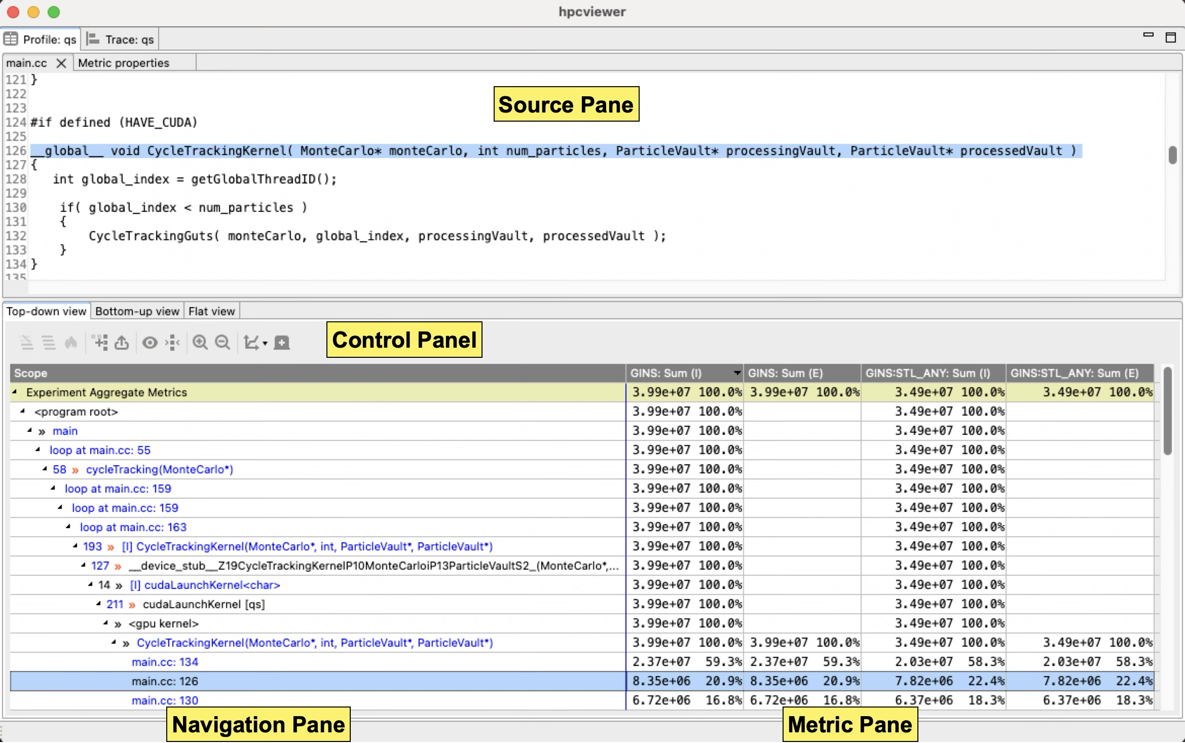
Figure Profile View above shows an annotated screenshot of hpcviewer’s user interface presenting a call path profile.
The annotations highlight hpcviewer’s principal window panes and key controls.
The Profile view is conceptually divided into two principal panes. The top pane is primarily to display source code associated with performance metrics, display metric properties, and plot graphs. The bottom pane contains a control panel, a navigation pane, and a metric pane, which associates performance metrics with code contexts displayed in the navigation pane. These panes are discussed in more detail in Section Panes.
hpcviewer displays calling-context-sensitive performance data in three views: Top-down, Bottom-up, and Flat View.
One selects the desired view by clicking on the corresponding view control tab.
We briefly describe the three views and their corresponding purposes.
Top-down View. This top-down view shows the dynamic calling contexts (call paths) in which costs were incurred. Using this view, one can explore performance measurements of an application in a top-down fashion to understand the costs incurred by calls to a procedure in a particular calling context. We use the term cost rather than simply time since
hpcviewercan present a multiplicity of metrics, such as cycles, cache misses, or derived metrics (e.g., cache miss rates or bandwidth consumed) that are other indicators of execution cost.
A calling context for a procedurefconsists of the stack of procedure frames active when the call was made tof. Using this view, one can readily see how much of the application’s cost was incurred byfwhen called from a particular calling context. If finer detail is of interest, one can explore how the costs incurred by a call tofin a particular context are divided betweenfitself and the procedures it calls. HPCToolkit’s call path profilerhpcrunand thehpcvieweruser interface distinguish calling context precisely by individual call sites; this means that if a proceduregcontains calls to procedurefin different places, these represent separate calling contexts.Bottom-up View. This bottom-up view enables one to look upward along call paths. The view apportions a procedure’s costs to its callers and, more generally, its calling contexts. This view is particularly useful for understanding the performance of software components or procedures used in multiple contexts. For instance, a message-passing program may call
MPI_Waitin many different calling contexts. The cost of any particular call will depend upon the structure of the parallelization in which the call is made. Serialization or load imbalance may cause long waits in some calling contexts, while other parts of the program may have short waits because computation is balanced and communication is overlapped with computation.
When several levels of the Bottom-up View are expanded, saying that it apportions metrics of a callee on behalf of its callers can be confusing. More precisely, the Bottom-up View apportions the metrics of a procedure on behalf of the various calling contexts that reach it.Flat View. This view organizes performance measurement data according to the static structure of an application. All costs incurred in any calling context by a procedure are aggregated in the Flat View. This complements the Top-down View, in which the costs incurred by a particular procedure are represented separately for each call to the procedure from a different calling context.
Panes#
hpcviewer’s browser window is divided into three panes: the Source pane, Navigation pane, and the Metrics pane.
We briefly describe the role of each pane.
Source Pane#
The source pane displays the source code associated with the current entity selected in the navigation pane.
When a performance database is first opened with hpcviewer, the source pane is initially blank because no entity has been selected in the navigation pane.
Selecting any entity in the navigation pane will cause the source pane to load the corresponding file and highlight the line corresponding to the selection.
Switching the source pane to display a different source file is accomplished by making another selection in the navigation pane.
Navigation Pane#
The navigation pane presents a hierarchical tree-based structure used to organize the presentation of an applications’s performance data. Entities in the navigation pane’s tree include load modules, files, procedures, procedure activations, inlined code, loops, and source lines. Selecting any of these entities will cause its corresponding source code (if any) to be displayed in the source pane. In this view, one can reveal or conceal children in this hierarchy by ‘opening’ or ‘closing’ any non-leaf (i.e., individual source line) entry.
The node in the tree will have the color blue if the source code is available. Otherwise, its color is black. If a node is a call statement, it will have the line number of the call statement (if the information is available) and the callee procedure as follows:
[
line_number] »callee
The symbol » represents a call to a procedure. For instance, the following node means that at line 1234 there is a call to function foo():
1234»foo()
Clicking the line number will display the source code at the call site of the function. Clicking the name of the called function will display the function’s first line.
The nature of the entities in the navigation pane’s tree structure depends upon whether one is exploring the Top-down View, the Bottom-up View, or the Flat View of the performance data.
In the Top-down View, entities in the navigation tree represent procedure activations, inlined code, loops, and source lines. While most entities link to a single location in source code, procedure activations link to two: the call site from which a procedure was called and the procedure itself.
In the Bottom-up View, entities in the navigation tree are procedure activations. Unlike procedure activations in the top-down view, in which call sites are paired with the called procedure, in the bottom-up view, call sites are paired with the calling procedure to allow to attribute the costs of a called procedure to multiple different call sites and callers. The node in this view has the following notation:
[
line_number] «caller
Where the symbol « represents a call by a procedure.
In the Flat View, entities in the navigation tree correspond to source files, procedure call sites (rendered the same way as procedure activations), loops, and source lines.
Control Panel#
The header above the navigation pane contains some controls for the navigation and metric view. In Figure Profile View, they are labeled as “navigation control.”
Flatten
 /
Unflatten
/
Unflatten  (Flat View only):
Enabling to flatten and unflatten the navigation hierarchy.
Clicking on the flatten button (the icon that shows a tree node with a slash through it) will replace each top-level scope shown with its children.
If a scope has no children (i.e., it is a leaf ), the node will remain in the view.
This flattening operation is useful for relaxing the strict hierarchical view so that peers at the same level in the tree can be viewed and ranked together.
For instance, this can be used to hide procedures in the Flat View so that outer loops can be ranked and compared to one another.
The inverse of the flatten operation is the unflatten operation, which causes an elided node in the tree to be made visible once again.
(Flat View only):
Enabling to flatten and unflatten the navigation hierarchy.
Clicking on the flatten button (the icon that shows a tree node with a slash through it) will replace each top-level scope shown with its children.
If a scope has no children (i.e., it is a leaf ), the node will remain in the view.
This flattening operation is useful for relaxing the strict hierarchical view so that peers at the same level in the tree can be viewed and ranked together.
For instance, this can be used to hide procedures in the Flat View so that outer loops can be ranked and compared to one another.
The inverse of the flatten operation is the unflatten operation, which causes an elided node in the tree to be made visible once again.Zoom-in
 /
Zoom-out
/
Zoom-out  :
Depressing the up arrow button will zoom in to show only information for the selected line and its descendants.
One can zoom out (reversing a prior zoom operation) by depressing the down arrow button.
:
Depressing the up arrow button will zoom in to show only information for the selected line and its descendants.
One can zoom out (reversing a prior zoom operation) by depressing the down arrow button.Hot call path
 :
This button automatically reveals and traverses the hot call path rooted at the selected node in the navigation pane with respect to the selected metric column. Let
:
This button automatically reveals and traverses the hot call path rooted at the selected node in the navigation pane with respect to the selected metric column. Let nbe the node initially selected in the navigation pane. A hot path fromnis traversed by comparing the values of the selected metric fornand its children. If one child accounts forT%or more (whereTis the threshold value for a hot call path) of the cost atn, then that child becomesnand the process repeats recursively.Add derived metric
 :
Create a new metric by specifying a mathematical formula.
See Section Derived Metrics for more details.
:
Create a new metric by specifying a mathematical formula.
See Section Derived Metrics for more details.Hide/show metrics
 :
Show or hide metric columns.
A metric property view will appear, and the user can select which metric columns should be displayed.
:
Show or hide metric columns.
A metric property view will appear, and the user can select which metric columns should be displayed.Resizing metric columns
 /
/
 :
Resize the metric columns based on either the width of the data or the width of both of the data and the column’s label.
:
Resize the metric columns based on either the width of the data or the width of both of the data and the column’s label.Export into a CSV format file
 :
Export the current metric table into a comma separated value (CSV) format file.
This feature only exports all metrics that are currently shown.
Metrics not shown in the view (whose scopes are not expanded) will not be exported (we assume these metrics are not significant).
:
Export the current metric table into a comma separated value (CSV) format file.
This feature only exports all metrics that are currently shown.
Metrics not shown in the view (whose scopes are not expanded) will not be exported (we assume these metrics are not significant).Increase font size
 /
Decrease font size
/
Decrease font size  :
Increase or decrease the size of the navigation and metric panes.
:
Increase or decrease the size of the navigation and metric panes.Show a graph of metric values
 (Top-down view only):
Show a graph (a plot, a sorted plot, or a histogram) of metric values associated with the selected node in CCT for all processes or threads (Section Plot Graphs).
(Top-down view only):
Show a graph (a plot, a sorted plot, or a histogram) of metric values associated with the selected node in CCT for all processes or threads (Section Plot Graphs).Show the metrics of a set of threads
 (Top-down view only):
Show the CCT and the metrics of a selected threads (Section Thread View).
(Top-down view only):
Show the CCT and the metrics of a selected threads (Section Thread View).
Metric Pane#
The metric pane displays one or more performance metrics associated with entities to the left in the navigation pane.
Entities in the tree view of the navigation pane are sorted at each level of the hierarchy by the metric in the selected column.
When hpcviewer is launched, the leftmost metric column is the default selection, and the navigation pane is sorted according to the values of that metric in descending order.
One can change the selected metric by clicking on a column header.
Clicking on the header of the selected column toggles the sort order between descending and ascending.
During analysis, one often wants to consider the relationship between two metrics. This is easier when the metrics of interest are in adjacent columns of the metric pane. One can change the order of columns in the metric pane by selecting the column header for a metric and then dragging it left or right to its desired position. The metric pane also includes scroll bars for horizontal scrolling (to reveal other metrics) and vertical scrolling (to reveal other scopes). Vertical scrolling of the metric and navigation panes is synchronized.
Understanding Metrics#
hpcviewer can present an arbitrary collection of performance metrics gathered during one or more runs, or compute derived metrics expressed as formulae. A derived metric may be specified with a formula that typically uses one or more existing metrics as terms in an expression.
For any given scope in hpcviewer’s three views, hpcviewer computes both inclusive and exclusive metric values.
First, consider the Top-down View.
Inclusive metrics reflect costs for the entire subtree rooted at that scope.
Exclusive metrics are of two flavors, depending on the scope.
For a procedure, exclusive metrics reflect all costs within that procedure but exclude callees.
In other words, for a procedure, costs are exclusive with respect to dynamic call chains.
For all other scopes, exclusive metrics reflect costs for the scope itself; i.e., costs are exclusive with respect to a static structure.
The Bottom-up and Flat Views contain inclusive and exclusive metric values relative to the Top-down View.
This means, e.g., that inclusive metrics for a particular scope in the Bottom-up or Flat View are with respect to that scope’s subtree in the Top-down View.
How Metrics are Computed#
Call path profile measurements collected by hpcrun correspond directly to the Top-down View.
hpcviewer derives all other views from exclusive metric costs in the Top-down View.
For the Bottom-up View, hpcviewer collects the cost of all samples in each function and attribute that to a top-level entry in the Bottom-up View.
Under each top-level function, hpcviewer can look up the call chain at all of the contexts in which the function is called.
For each function, hpcviewer apportions its costs among each of the calling contexts in which they were incurred.
hpcviewer computes the Flat View by traversing the calling context tree and attributing all costs for a scope to the scope within its static source code structure.
The Flat View presents a hierarchy of nested scopes for load modules, files, procedures, loops, inlined code, and statements.
Example#
Assume one has a simple recursive program divided into two source files file1.c and file2.c as follows:
// file1.c
f () {
  g ();
}
// m is the main routine
m () {
  f ();
  g ();
}
// file2.c
// g can be a recursive function
g () {
  if ( . . ) g ();
  if ( . . ) h ();
}

h () {
}
Figure Top-down View below shows the top-down representation of the above program where procedure m is the main entry program, which then calls two procedures: f and g.
Routine g can behave as a recursive function depending on the value of the condition branch (lines 3–4).
In this figure, we use numerical subscripts to distinguish between different instances of the same procedure.
In contrast, in Bottom-up View and Flat View, we use alphabetic subscripts.
We use different labels because there is no natural one-to-one correspondence between the instances in the different views.
Top-down View |
|---|
|
Each node of the tree has three boxes: the left-most is the name of the node (or in this case the name of the procedure, the center is the inclusive metric cost, and on the right is the exclusive cost. |
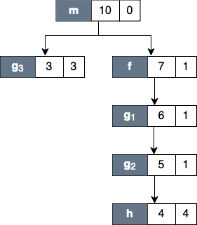
Figure Top-down View above shows an example of the call chain execution of the program annotated with both inclusive and exclusive costs. Computation of inclusive costs from exclusive costs in the Top-down View involves simply summing up all of the costs in the subtree below.
In this figure, we can see that on the right path of the routine m, routine g (instantiated in the diagram as g_1) performed a recursive call (g_2) before calling routine h.
Although g_1, g_2 and g_3 are all instances from the same routine (i.e., g), we attribute a different cost for each instance.
This separation of cost can be critical to identify which instance has a performance problem.
Bottom-up View |
|---|
|
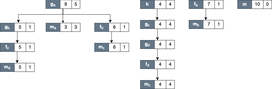
Figure Bottom-up View shows the corresponding scope structure for the Bottom-up View and the costs we compute for this recursive program.
The procedure g noted as g_a (which is a root node in the diagram), has different cost to g as a callsite as noted as g_b, g_c and g_d.
For instance, on the first tree of this figure, the inclusive cost of g_a is 9, which is the sum of the highest cost for each path in the Top-down View that includes g: the inclusive cost of g_3 (which is 3) and g_1 (which is 6).
We do not attribute the cost of g_2 here since it is a descendant of g_1 (in other term, the cost of g_2 is included in g_1).
Flat View |
|---|
|
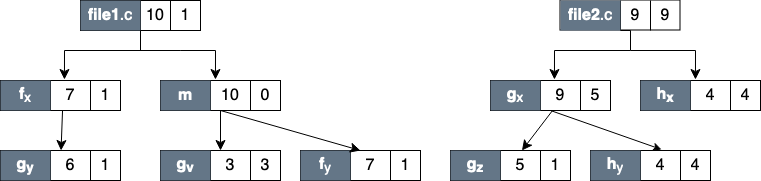
Inclusive costs need to be computed similarly in the Flat View.
The inclusive cost of a recursive routine is the sum of the highest cost for each branch in calling context tree.
For instance, in Figure Flat View, The inclusive cost of g_x, defined as the total cost of all instances of g, is 9, and this is consistently the same as the cost in the bottom-up tree.
The advantage of attributing different costs for each instance of g is that it enables a user to identify which instance of the call to g is responsible for performance losses.
Derived Metrics#
Frequently, the data become useful only when combined with other information such as the number of instructions executed or the total number of cache accesses.
While users don’t mind a bit of mental arithmetic and frequently compare values in different columns to see how they relate to a scope, doing this for many scopes is exhausting.
To address this problem, hpcviewer provides a mechanism for defining metrics.
A user-defined metric is called a “derived metric.”
A derived metric is defined by specifying a spreadsheet-like mathematical formula that refers to data in other columns in the metric table by using $n to refer to the value in the nth column.
Formulae#
The formula syntax supported by hpcviewer is inspired by spreadsheet-like in-fix mathematical formulae.
Operators have standard algebraic precedence.
Examples#
Suppose the database contains information from five executions, where the same two metrics were recorded for each:
Metric 0, 2, 4, 6 and 8: total number of cycles
Metric 1, 3, 5, 7 and 9: total number of floating point operations
To compute the average number of cycles per floating point operation across all of the executions, we can define a formula as follows:
avg($0, $2, $4. $6. $8) / avg($1, $3, $5, $7, $9)
Creating Derived Metrics#
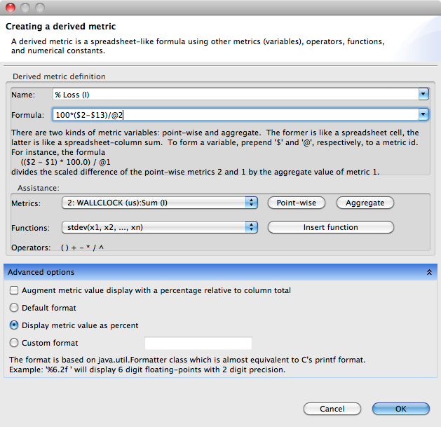
A derived metric can be created by clicking the Derived metric tool item in the navigation/control pane. A derived metric window will then appear as shown in Figure Derived Metric below.
Derived metric dialog box |
|---|
|
The window has two main parts:
Derived metric definition:
New name for the derived metric. Supply a string that will be used as the column header for the derived metric.
Formula definition field. In this field, the user can define a formula with a spreadsheet-like mathematical formula. A user can type a formula into this field, or use the buttons in Metrics pane below to help insert metric terms or function templates.
Metrics. This is used to find the ID of a metric. For instance, in this snapshot, the metric
WALLCLOCKhas the ID2.Point-wisebutton will insert the metric ID with a “dollar” character ($) in the formula field. This dollar prefix refers to the metric value at an individual node in the calling context tree (point-wise) or the value at the root of the calling context tree (aggregate).Aggregatebutton will insert the metric ID with prefix “at” character (@) in the formula field. This prefix refers to the aggregate (root) value of the metric.
Functions. This is to guide the user who wants to insert functions in the formula definition field. Some functions require only one metric as the argument, but some can have two or more arguments. For instance, the function
avg()which computes the average of some metrics, needs at least two arguments.
Advanced options:
Augment metric value display with a percentage relative to column total. When this box is checked, each scope’s derived metric value will be augmented with a percentage value, which for scope s is computed as the 100 * (s’s derived metric value) / (the derived metric value computed by applying the metric formula to the aggregate values of the input metrics for the entire execution). Such a computation can lead to nonsensical results for some derived metric formulae. For instance, if the derived metric is computed as a ratio of two other metrics, the aforementioned computation that compares the scope’s ratio with the ratio for the entire program won’t yield a meaningful result. To avoid a confusing metric display, think before you use this button to annotate a metric with its percent of the total.
Default format. This option will display the metric value using scientific notation with three digits of precision, which is the default format.
Display metric value as percent. This option will display the metric value formatted as a percent with two decimal digits. For instance, if the metric has a value
12.3415678, with this option, it will be displayed as12.34%.Custom format. This option will present the metric value with your customized format. The format is equivalent to Java’s Formatter class, or similar to C’s printf format. For example, the format “
%6.2f” will display six-digit floating-points with two digits to the right of the decimal point.
Note that the entered formula and the metric name will be stored automatically. One can then review again the formula (or metric name) by clicking the small triangle of the combo box.
Metrics in Execution-context level#
Execution context is an abstract concept of a measurable code execution. For example, in a pure MPI application, an execution context is an MPI rank, while an execution context of an OpenMP application is an OpenMP thread, and an execution context of GPU applications can be a GPU stream. For hybrid MPI+OpenMP applications, its execution context is its MPI rank and its OpenMP master and worker threads.
There are two types of execution context:
Physical which represents the hardware ID of the execution, such as:
NODE: the ID of the compute node.CORE: the CPU core to which the application thread is bound.
Logical which represents any non-physical entity of the program execution, like:
RANK: the rank of the process (like the MPI process),THREAD: the application CPU thread (such as OpenMP thread),GPUCONTEXT: the context used to access a GPU (like a GPU device), andGPUSTREAM: a stream or queue used to push work to a GPU.
Plot Graphs#
Plot graph |
|---|
|
Plot graph view of a procedure in GAMESS MPI+OpenMP application showing an imbalance where a group of execution contexts have much higher GPU operations than others. |
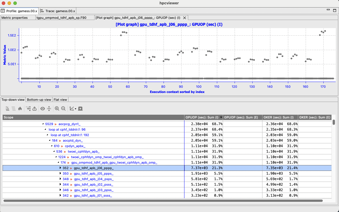
HPCToolkit Experiment databases that have been generated by hpcprof can be used by hpcviewer to plot graphs of metric values for each execution context.
This is particularly useful for quickly assessing load imbalance in context across the several threads or processes of an execution.
Figure Plot graph shows hpcviewer rendering such a plot.
The horizontal axis shows the application execution context sorted by index (in this case, it’s MPI rank and OpenMP thread).
The vertical axis shows metric values for each execution context.
Because hpcviewer can generate scatter plots for any node in the Top-down View, these graphs are calling-context sensitive.
To create a graph, first select a scope in the Top-down View; in the Figure Plot graph, the procedure gpu_tdhf_apb_j06_pppp_ is selected.
Then, click the graph button to show the associated sub-menus.
At the bottom of the sub-menu is a list of non-empty metrics for the selected scope.
Each metric contains a sub-menu that lists the three different types of graphs:
Plot graph: This standard graph plots metric values ordered by their execution context.
Sorted plot graph: This graph plots metric values in ascending order.
Histogram graph: This graph is a histogram of metric values. It divides the range of metric values into a small number of sub-ranges. The graph plots the frequency of the metric that falls into a particular sub-range.
Remark that the label of execution context for a mixed programming model program like a hybrid MPI and OpenMP (Figure Plot graph) is
PROCESS . THREAD
Hence, if the application is a hybrid MPI and OpenMP program, and the execution contexts are 0.0, 0.1, … 31.0, 31.1 it means MPI process 0 has two threads: thread 0 and thread 1 (similarly with MPI process 31).
The viewer also provides additional functionalities by right-clicking on the graph to display the context menus:
Adjust Axes Ranges: to reset the axis X, Y, or both.
Zoom In/Out: to zoom-in or zoom-out the current graph.
Save As: to save the current graph to a file in
*.pngor.jpegformat.Properties: to change the settings of the current graph. This setting is not persistent.
Display …: this menu is only enabled if one right-click on the dot of the graph. It allows to display the Thread view of the specific execution context.
In a graph of metrics for a calling context, hovering over a dot in the graph will display the metric value and the name of its associated execution context.
In the Profile view, metrics for a GPU operation are attributed to either the main thread under <program root> or aggregated under <thread root> for operations launched by a thread with an id > 0. In the graphical thread view, each thread displays its value for the GPU metric associated with the calling context.
Note:
Currently, it is only possible to generate scatter plots for metrics directly collected by
hpcrun, which excludes derived metrics created withinhpcviewer.
Thread View#
hpcviewer can also displays the metrics of certain execution contexts (threads and/or processes) named Thread View.
To select a set of execution contexts, one needs to use the execution-context selection window by clicking button from the control panel in the Top-down view.
Selecting execution contexts |
|---|
|
A snapshot of an execution-contexts selection window. One can refine the list of execution contexts using regular expression by selecting the Regular expression checkbox. |
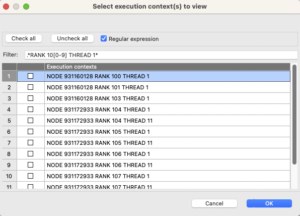
On the Execution-context selection window, one needs to select the checkbox of the execution context of interest. To narrow the list, one can specify the thread name on the filter part of the window. For instance for a hybrid MPI and OpenMP application, to display just the main thread (thread zero), one can type:
THREAD 0
on the filter, and the view only lists all threads 0, such as RANK 1 THREAD 0, RANK 2 THREAD 0, and RANK 3 THREAD 0.
Once execution contexts have been selected, one can click OK, and the Thread View will be activated. The tree of the view is the same as the tree from the Top-down view, with the metrics only from the selected execution contexts. If there is more than one execution context, the metric value is the sum of the values of the selected execution contexts.
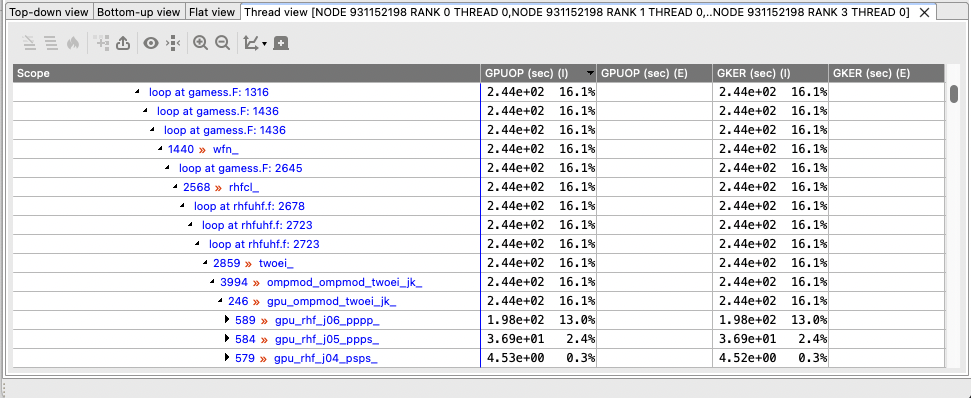
Threads view contains a CCT and metrics of a set of threads |
|---|
|
Example of Thread View which displays a set of execution contexts. The first column is a calling-context tree (CCT) equivalent to the CCT in the Top-down View. The next columns represent the metrics from the selected execution contexts (in this case, they are the sum of metrics from rank 0 threads 0 to rank 3 thread 0) |
Filtering Tree Nodes#
Occasionally, It is useful to omit uninterested nodes of the tree to enable to focus on important parts.
For instance, you may want to hide all nodes associated with OpenMP runtime and just show all nodes and metrics from the application.
For this purpose, hpcviewer provides filtering to elide nodes that match a filter pattern.
hpcviewer allows users to define multiple filters, and each filter is associated with a glob pattern and a type.
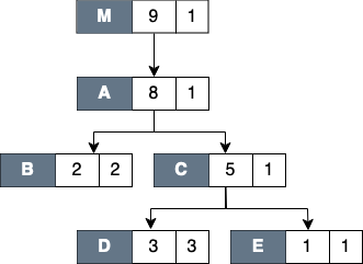
The figures below show examples of applying a filter mode. In these figures, each node is attributed with three boxes: the node label (left), the inclusive cost (middle) and the exclusive cost (right).
Original CCT |
Filtering with “self only” mode |
|---|---|
|
|
The original top-down tree (or CCT) without any filters. |
The result of applying self only filter on node |
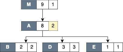
There are three types of filter: “self only” to omit matched nodes, “descendants only” to exclude only the subtree of the matched nodes, and “self and descendants” to remove matched nodes and its descendants.
- Self only
This filter is useful to hide intermediary runtime functions such as pthread or OpenMP runtime functions. All nodes that match filter patterns will be removed, and their children will be augmented to the parent of the elided nodes. The exclusive cost of the elided nodes will be also augmented into the exclusive cost of the parent of the elided nodes. Figure Filter self shows the result of filtering node
Cof the CCT from Figure 10.10. After filtering, nodeCis elided and its exclusive cost is augmented into the exclusive cost of its parent (nodeA). The children of nodeC(nodesDandE) are now the children of nodeA.- Descendants only
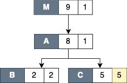
This filter elides only the subtree of the matched node, while the matched node itself is not removed. A common usage of this filter is to exclude any call chains after MPI functions. As shown in Figure Filter descendants, filtering node
Cincurs nodesDandEto be elided and their exclusive cost is augmented to nodeC.- Self and descendants
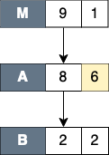
This filter elides both the matched node and its subtree. This type is useful to exclude any unnecessary details such as glibc or malloc functions. Figure Filter self and descendants shows that filtering node
Cwill elide the node and its children (nodesDandE). The total of the exclusive cost of the elided nodes is augmented to the exclusive cost of nodeA.
Filtering with “descendants only” mode |
Filtering with “self and descendants” mode |
|---|---|
|
|
The result of applying Descendants only filter on node |
The result of applying self and descendants filter on node |
The filter feature can be accessed by clicking the menu “Filter” and then submenu “Show filter property”, which will then show the Filter window as shown below:
Filter window |
|---|
|
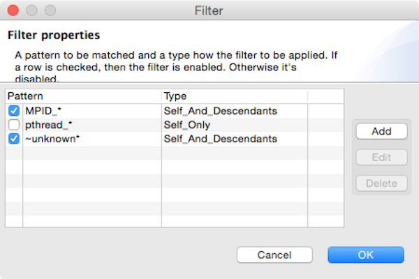
The window consists of a table of filters and a group of action buttons: add to create a new filter, edit to modify a selected filter, and delete to remove a set of selected filters. The table comprises two columns: the left column is to display a filter’s switch whether the filter is enabled or disabled, and a glob-like filter pattern; and the second column is to show the type of pattern (self only, children only or self and children). If a checkbox is checked, it signifies the filter is enabled; otherwise, the filter is disabled.
Cautious is needed when using the filter feature since it can change the tree’s shape, thus affecting the interpretation of performance analysis.
Furthermore, if the filtered nodes are children of a “root” node (such as <program root> and <thread root>), the exclusive metrics in Bottom-up and flat view can be misleading.
Note that the filter set is global: it affects all open databases in all windows, and it is persistent that it will also affect across hpcviewer sessions.
Convenience Features#
In this section we describe some features of hpcviewer that help improve productivity.
Source Code Pane#
The pane is used to display a copy of your program’s source code or HPCToolkit’s performance data in XML format; for this reason, it does not support editing of the pane’s contents.
To edit a program source code, one should use a favorite editor to edit the original copy of the source, not the one stored in HPCToolkit’s performance database.
Thanks to built-in capabilities in Eclipse, hpcviewer supports some useful shortcuts and customization:
Find. To search for a string in the current source pane,
ctrl-f(Linux and Windows) orcommand-f(Mac) will bring up a find dialog that enables you to enter the target string.Copy. To copy a selected text into the system’s clipboard by pressing
ctrl-con Linux and Windows orcommand-con Mac.
Metric Pane#
For the metric pane, hpcviewer has some convenient features:
Sorting the metric pane contents by a column’s values. First, select the column to sort. If no triangle appears next to the metric, click again. A downward pointing triangle means that the rows in the metric pane are sorted in descending order according to the column’s value. Additional clicks on the header of the selected column will toggle back and forth between ascending and descending.
Changing column width. To increase or decrease the width of a column, first put the cursor over the right or left border of the column’s header field. The cursor will change into a vertical bar between a left and right arrow. Depress the mouse and drag the column border to the desired position.
Changing column order. If it would be more convenient to have columns displayed in a different order, they can be permuted. Depress and hold the mouse button over the header of column to move and drag the column right or left to its new position.
Copying selected metrics into a clipboard. To copy selected lines of scopes/metrics, one can right-click on the metric pane or navigation pane and then select the menu Copy. The copied metrics can then be pasted into any text editor.
Hiding or showing metric columns. Sometimes, it may be more convenient to suppress the display of metrics that are not of current interest. When there are too many metrics to fit on the screen at once, it is often useful to suppress the display of some. The icon
above the metric pane will bring up the metric property pane on the source pane area.The pane contains a list of metrics sorted according to their order in HPCToolkit’s performance database for the application. Each metric column is prefixed by a check box to indicate if the metric should be displayed (if checked) or hidden (unchecked). To display all metric columns, one can click the Check all button. A click to Uncheck all will hide all the metric columns. The pane also allows to edit the name of the metric or change the formula of a derived metric. If the metric has no cost, it will be marked with a grey color, and it isn’t editable.
Finally, an option
Apply to all viewswill set the configuration into all views (Top-down, Bottom-up, and Flat views) when checked. Otherwise, the configuration will be applied only on the current view.
Trace view#
Trace view (Tallent et al. 2011) is a time-centric user interface for interactive examination of a sample-based time series (hereafter referred to as a trace) view of a program execution. Trace view can interactively present a large-scale execution trace without concern for the scale of parallelism it represents.
To collect a trace for a program execution, one must instruct HPCToolkit’s measurement system to collect a trace.
When launching a dynamically-linked executable with hpcrun, add the -t flag to enable tracing.
When collecting a trace, one must also specify a metric to measure. The best way to collect a useful trace is to asynchronously sample the execution with a time-based metric such as REALTIME, CYCLES, or CPUTIME.
Trace dimensions |
|---|
|
The logical view of traces of call-path samples on three dimensions: time, execution context (rank/thread/GPU), and call stack (also known as call-path). |
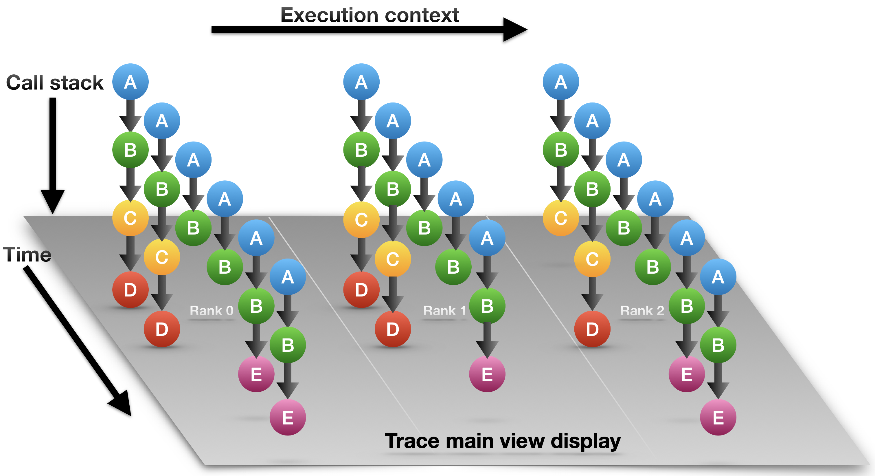
As shown in the Trace dimensions figure above, call-path traces consist of data in three dimensions: execution context (also called profile) representing a process or a thread rank or a GPU stream, time, and call stack.
A crosshair in Trace view is defined by a triplet (p,t,d) where p is the selected process/thread rank, t is the selected time, and d is the selected call stack depth.
Trace view renders a view of processes and threads over time. The Depth View shows the call stack depth over time for the thread selected by the cursor. Trace view’s Call-stack View shows the call stack associated with the thread and time pair specified by the cursor. Each of these views plays a role in understanding an application’s performance.
In the Trace view, each procedure is assigned a specific color. The Trace dimensions figure above shows that at depth 1, each call stack has the same color: blue. This node represents the main program that serves as the root of the call chain in all processes at all times. At depth 2, all processes have a green node, which indicates another procedure. At depth 3, in the first time step, all processes have a yellow node; in subsequent time steps, they have purple nodes. This might indicate that the processes are first observed in an initialization procedure (represented by yellow) and later observed in a solve procedure (represented by purple). The pattern of colors that appears in a particular depth slice of the Main View enables a user to visually identify inefficiencies such as load imbalance and serialization.
Trace view with legends |
|---|
|
A snapshot of traces of an MPI+OpenMP program. The main view shows the Rank or Execution context as the Y-axis and the program execution time as the X-axis. |
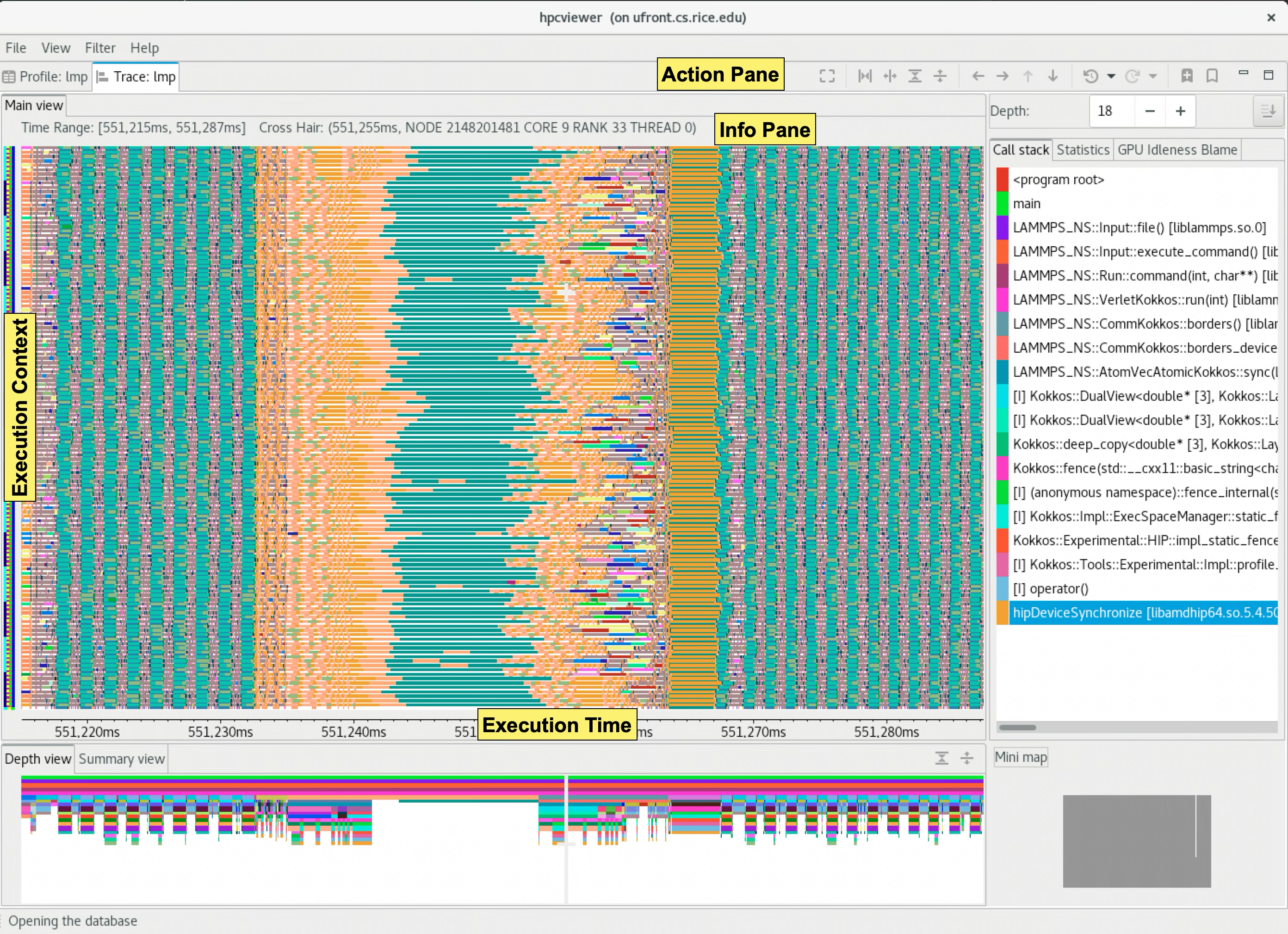
The above Trace view figure highlights Trace view’s four principal window panes: Main View, Depth View, Call Stack View, and Mini Map View, while the Trace view figure below shows two additional window panes: Summary View and Statistics View:
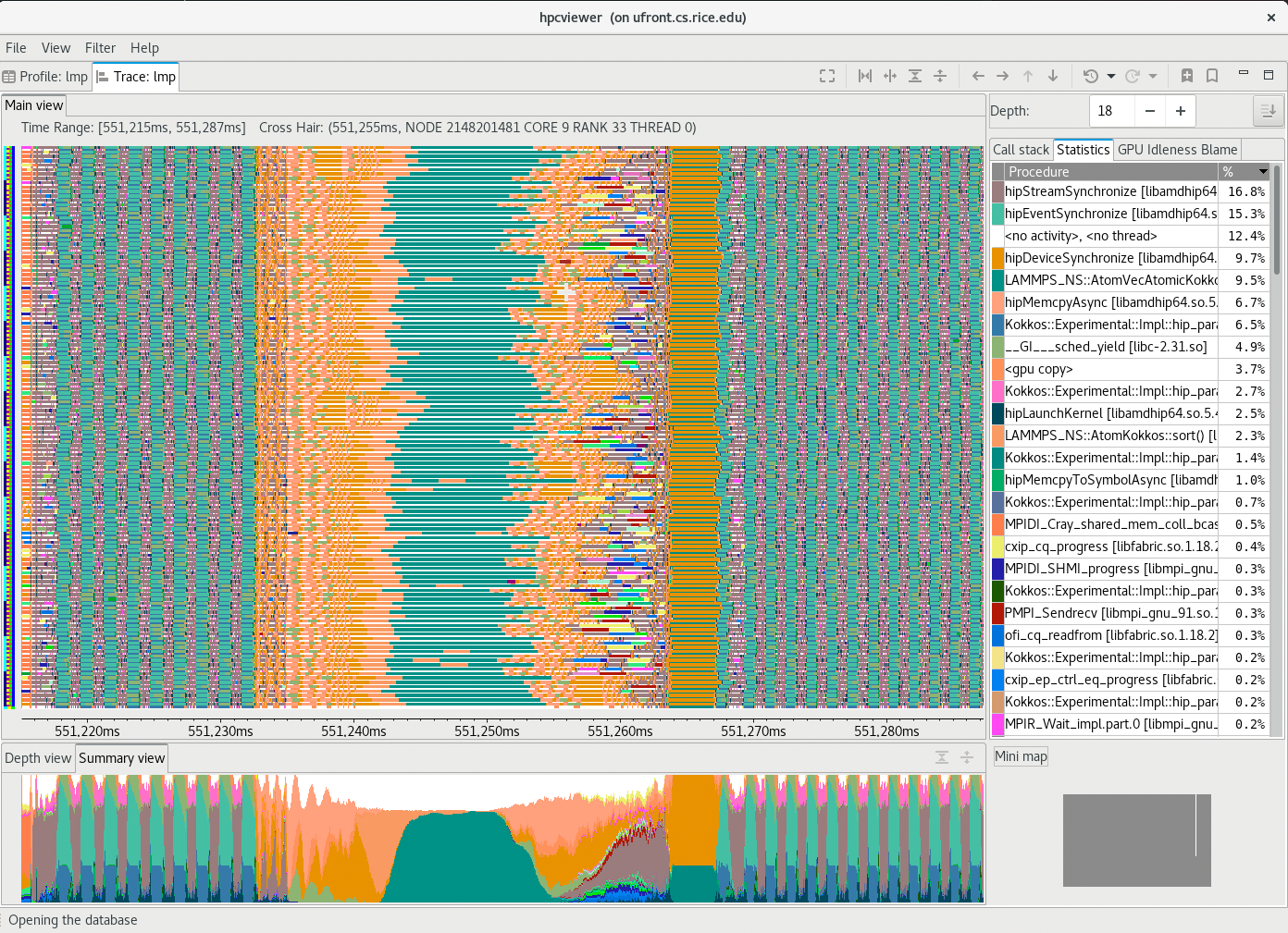
Trace view with the Summary View and Statistics View |
|---|
|
A screenshot of |
Main View (top tab, left pane): This is the Trace view’s primary view. This view shows time on the horizontal axis and the execution context (rank, thread, GPU stream) on the vertical axis; time moves from left to right. Compared to typical process/time views, there is one key difference. The view is a user-controllable slice of the execution-context/time/call-stack space to show the call stack hierarchy (see the Trace dimensions figure). Given a call-stack depth, the view shows the color of the currently active procedure at a given time and process rank. (If the requested depth is deeper than a particular call stack, then Trace view simply displays the deepest procedure frame and, space permitting, overlays an annotation indicating the fact that this frame represents a shallower depth.)
Trace View assigns colors to procedures based on (static) source code procedures. Thus, the same color within the Main and Depth views refers to the same procedure.
The Main view has a white crosshair representing a selected time and process space. For this selected point, the Call Stack View shows the corresponding call stack, while the Depth View shows the selected process.
Depth View (bottom tab, left pane): The view presents a <call-path, time> dimension for the current execution context selected by the Main view’s crosshair. It shows for each virtual time along the horizontal axis a stylized call stack along the vertical axis, where ‘main’ is at the top and leaves (samples) are at the bottom. In other words, this view shows for the whole time range, in a qualitative fashion, what the Call Path View shows for a selected point. The horizontal time axis aligns exactly with the Trace View’s time axis; and the colors are consistent across both views. This view has a crosshair corresponding to the currently selected time and call stack depth. One can specify a new crosshair time and a new time range:
Selecting a new crosshair time
tcan be done by clicking a pixel within Depth View. This will update the crosshair in Main View and the call path in Call Stack View.Selecting a new time range [
t_m,t_n] = {t|t_m<=t<=t_n} is performed by first clicking the position oft_mand dragging the cursor to the position oft_n. A new content in Depth View and Main View is then updated. Note that this action will not update the call path in Call Stack View since it does not change the position of the crosshair.
Summary View (bottom tab, left pane): The view shows the proportion of each subroutine within the current time range. Similar to the Depth view, the Summary view’s time range reflects the Trace view’s time range…
Call Stack View (top tab, right pane): This view shows two things:
the current call stack depth that defines the hierarchical slice shown in the Trace view, and
the actual call stack for the point selected by the Trace view’s crosshair. To easily coordinate the call stack depth value with the call path, the Call Stack View currently suppresses details such as loop structure and call sites; we may use indentation or other techniques to display this in the future. In this view, the user can select the depth dimension of the Main view by either typing the depth in the depth editor or selecting a procedure in the Call stack view.
Statistics View (top tab, right pane, not shown): This view shows the list of procedures active in the space-time region shown in the Main view at the current call stack depth. Each procedure’s percentage in the Statistics view indicates the percentage of pixels in the Main view pane filled with this procedure’s color at the current Call stack depth. When the Main view is navigated to show a new time-space interval or the call-stack’s depth is changed, the statistics view will update its list of procedures and the percentage of execution time to reflect the new space-time interval or depth selection.
GPU Idleness Blame View (top tab, right pane, not shown): The view is only available if the database contains information on GPU traces. It shows the list of procedures that cause GPU idleness displayed in the trace view. If the trace view displays one CPU thread and multiple GPU streams, then the CPU thread will be blamed for the idleness of those GPU streams. If the view contains more than one CPU thread and multiple GPU streams, then the cost of idleness is shared among the CPU threads.
Mini Map View (bottom tab, right pane): The Mini Map shows, relative to the process/time dimensions, the portion of the execution shown by the Trace View. The Mini Map enables one to zoom and to move from one close-up to another quickly. The user can also move the current selected region to another region by clicking the white rectangle and dragging it to the new place.
Action and Information Pane#
Main View is divided into two parts: the top part, which contains action and information panes, and the main canvas, which displays the traces.
The buttons in the action pane are the following:
Home
 : Resetting the view configuration into the original view, i.e., viewing traces for all times and processes.
Horizontal zoom in
 / out
/ out  : Zooming in/out the time dimension of the traces.
Vertical zoom in
 / out
/ out  : Zooming in/out the process dimension of the traces.
Navigation buttons
 ,
,  ,
,  ,
,  : Navigating the trace view to the left, right, up and bottom, respectively. It is also possible to navigate with the arrow keys in the keyboard. Since Main View does not support scroll bars, the only way to navigate is through navigation buttons (or arrow keys).
Undo
 : Canceling the action of zoom or navigation and returning back to the previous view configuration.
Redo
 : Redoing of previously undo change of view configuration.
Save
 / Open
  a view configuration : Saving/loading a saved view configuration.
A view configuration file contains information about the process/thread and time ranges shown, the selected depth, and the position of the crosshair.
It is recommended that the view configuration file be stored in the same directory as the database to ensure that it matches the database since a configuration does not store its associated database. Although it is possible to open a view configuration file associated with a different database, it is not recommended since each database has different time/process dimensions and depth.
a view configuration : Saving/loading a saved view configuration.
A view configuration file contains information about the process/thread and time ranges shown, the selected depth, and the position of the crosshair.
It is recommended that the view configuration file be stored in the same directory as the database to ensure that it matches the database since a configuration does not store its associated database. Although it is possible to open a view configuration file associated with a different database, it is not recommended since each database has different time/process dimensions and depth.
At the top of an execution’s Main View pane is information about the data shown in the pane.
Time Range. It shows the time interval of the Main view along the horizontal dimension.
Cross Hair. It indicates the current cursor position in the time and execution-context dimensions.
Customizing the Color Map#
Trace view allows users to customize the color of a specific procedure or a group of procedures.
To do that, one can select the View - Color map menu, and Color Map window will appear as shown below:
Color map window |
|---|
|
This snapshot shows that any procedure names that match with “ |
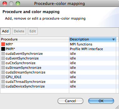
To add a new procedure-color map, click the Add button and a Color map window will appear.
In this window, one can specify the procedure’s name or a glob pattern of procedure, and then specify the color to be associated by clicking the color button.
Clicking OK will close the window and add the new color map to the global list.
Note that this map is persistent across sessions, and will apply to other databases as well.
Filtering Execution Contexts#
One can select which execution contexts (ranks, threads or GPU streams) to be displayed in Trace View, by selecting the Filter - execution contexts menu.
This will display a filter window that allows to select which execution contexts to show/hide:
Filter execution context window |
|---|
|
An example of narrowing the list of execution contexts using both a regular expression and the minimum number of samples criteria |
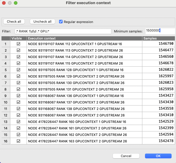
Similar to Profile View’s thread selection, one can narrow the list by specifying the name of the execution context on the filter part of the window. In addition, one can also narrow the list based on the minimum number of trace samples (the third column of the table), as shown by the above figure.
Filtering Suggestions#
Sometimes, it is helpful to associate a group of procedures (such as
MPI_*) to a specific color to approximate its statistic percentage.Filtering GPU traces: use the filter menu to select what execution traces to see
CPU only, GPU, or a mix: type a string or a regular expression in the chooser to select or unselect the a set of execution contexts
only traces that exceed a minimum number of samples
Filtering GPU calling context tree nodes: to hide clutter
hide individual CCT nodes: e.g. lines that have no source code mapping
library@0x0f450hide subtrees: e.g., MPI implementation or implementation of CUDA primitives
Trace view also provides a context menu by right-clicking on the view to save the current display. This context menu is also available on the Depth view and the Summary view.
Accessing Remote Databases#
hpcviewer can open performance databases located on remote hosts. Access to performance data on a remote host is supported by running a utility known as hpcserver on the remote host to communicate with an instance of hpcviewer running elsewhere.
With the help of an instance of hpcserver, a user running hpcviewer can interact with a remote database in real-time, viewing and analyzing performance metrics.
Protecting against unauthorized access was a principal design goal of hpcviewer’s capability for remote access to performance data.
Several aspects of the design work together to prevent unauthorized access to data on a remote system.
Before accessing data on a remote host, a local instance of
hpcviewermust authenticate with an instance ofhpcserverrunning on the remote host using standard mechanisms (e.g. password, ssh keys).Communication between
hpcviewerand an instance ofhpcserveroccurs over an SSH tunnel. This guarantees that all communication betweenhpcviewerandhpcserveris encrypted, safeguarding it from unauthorized access or tampering.To further safeguard communication, an instance of
hpcserverlaunched by an authenticated user uses a UNIX domain socket only accessible to that user when communicating with an instance ofhpcviewer. This prevents access to the socket by other users.hpcviewerdoesn’t save a copy of remote performance data to the local file system, which reduces the risk of unauthorized access to the data.
To enable remote access to data on a host, one needs to build and install hpcserver on the host, as described in the next section.
Building and Installing hpcserver#
hpcserver supports secure and efficient communication between a server containing an HPCToolkit database and an instance of hpcviewer running elsewhere. hpcserver is written entirely in Java and is designed for cross-platform compatibility. Below are the requirements and instructions for building and installing hpcserver.
Requirements:
Java 17 or newer
Maven 3.8.4 or newer
Build and install:
Checkout the
mainbranch ofhpcserver:git clone https://gitlab.com/hpctoolkit/hpcserver git checkout main
Build using Maven
mvn clean package
Install to a directory with the
install.shscript./scripts/install.sh -j /path/to/java-jdk/root /path/where/to/install/hpcserver
install.sh supports an optional -f argument, which forces an installation by skipping Java sanity checks.
Tip
Always use the
-j /path/to/java-jdk/rootarguments when installinghpcserver. Just becausejavais on your path doesn’t guarantee that it will be on the path of anyone trying to launch an instance ofhpcserver.When installing
hpcserver, make sure that the/path/to/java-jdk/rootis accessible to anyone who will be connecting to the platform withhpcviewerto launch an instance ofhpcserverFor the convenience of users,
/path/where/to/install/hpcservershould be short because remote users will need to type the path into a remote instance ofhpcviewer. If convenient,/path/where/to/install/hpcservercan be/path/to/hpctoolkit-installation
Opening a Remote Database#
Steps to opening a remote database:
Click the menu
File-Open remote databaseOn Remote connection window, type the required fields:
Remote connection window
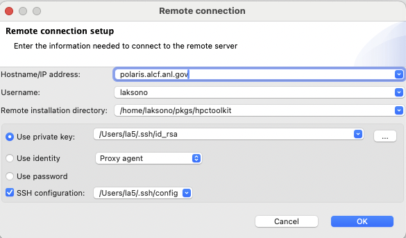
Hostname/IP address: the name of the remote host where
hpcserveris installedUsername: the username at the remote host
Remote installation directory: the absolute path of
hpcserverinstallation. In the above case, it’s/path/hpctoolkit
To facilitate the connection,
hpcviewerallows to connect via three options:Use private key: use SSH private key whenever possible. This is the recommended way to avoid typing the password all the time.
Use identity: use SSH identity. This is an experimental feature to connect via user’s SSH identity.
Use password: use a password to connect. One can check this option if using a private key is problematic.
SSH configuration: use the user’s SSH configuration to simplify the connection to a remote host that requires multiple hops or proxy jump. Usually the configuration file is located at
$HOME/.ssh/configon most POSIX platforms.
Once the configuration is set, one needs to click the
OKbutton to start the connection.If the connection succeeds, one has to choose an HPCToolkit database from the Remote database browser window. The window shows the current remote directory at the top, and the list of its content:
Remote database browser window
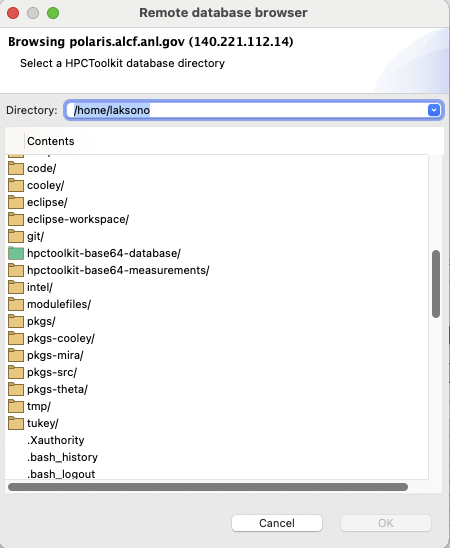
 icon represents a regular directory, and one can access it via double-click at the icon or the name of the folder.
 icon represents an HPCToolkit database. Selecting this item will enable the
 OKbutton.A no icon item represents a regular file.
Note: the
OKbutton will remain disabled until one selects an HPCToolkit database.